[Titanic] Feature Engineering(1) - 결측값(Null) 처리
728x90
반응형
※ 타이타닉에 승선한 사람들의 데이터로 승객들의 생존여부를 예측하는 모델 구축 / 개발
※ Dataset Check, EDA 이후 Feature Engineering 과정을 통해 모델 학습도와 성능 향상
- Null값 채우기(Age, Embarked), 카테고리화(Age)
- Feature Engineering은 모델의 학습과 성능도(=정확도)를 높이기 위해 학습 데이터의 패턴이 잘 보일 수 있도록 수정하여 Target값을 잘 예측(predict)할 수 있도록 하는 중요한 과정이다.
- 각 Feature의 특성에 맞는 엔지니어링 작업을 수행
1. 결측값(Null) 채우기
1.1. Age, Name → Initial 로 치환 후 Null 채우기
- Name이 탑승객별로 너무 상이하여, 이름에 있는 타이틀(Mr, Miss)를 그룹으로 나누어서 'Initial' 이라는 Feature 생성
- 그리고 그 Initial 그룹의 나이 평균값을 산출해서 해당하는 Null값으로 채운다
# 'Age' Feature 내 Null값의 총량 확인
- Age의 Null값은 총 177개 확인
df_train['Age'].isnull().sum()
>>
177
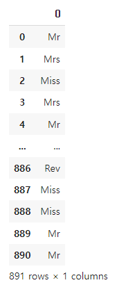
# Name 데이터 출력 (상위 10개까지)
df_train['Name'][:10]
>>
0                              Braund, Mr. Owen Harris
1    Cumings, Mrs. John Bradley (Florence Briggs Th...
2                               Heikkinen, Miss. Laina
3         Futrelle, Mrs. Jacques Heath (Lily May Peel)
4                             Allen, Mr. William Henry
5                                     Moran, Mr. James
6                              McCarthy, Mr. Timothy J
7                       Palsson, Master. Gosta Leonard
8    Johnson, Mrs. Oscar W (Elisabeth Vilhelmina Berg)
9                  Nasser, Mrs. Nicholas (Adele Achem)
Name: Name, dtype: object
# Name에서 타이틀(Mr, Mrs 등) 추출하기 - extract 함수
- extract() : 정규 표현식에 맞는 추출해주는 함수
df_train['Name'].str.extract('([A-Za-z]+)\.')
>>
# 바로 위에서 추출한 타이틀을 'initial' 이라는 Feature를 생성해서 저장
df_train['Initial'] = df_train['Name'].str.extract('([A-Za-z]+)\.')
df_test['Initial'] = df_test['Name'].str.extract('([A-Za-z]+)\.')
# Name의 타이틀별 남자/여자의 성별 구분 - Table과 시각화 출력
pd.crosstab(df_train['Initial'], df_train['Sex']).T.style.background_gradient(cmap='winter')
>>
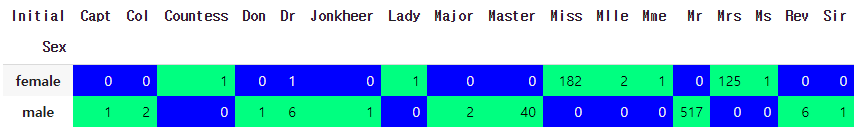
# 간단한 그룹으로 치환 - replace() 함수 사용
- 타이틀의 종류가 많으므로, 간단하게 'Mr, Mrs, Miss, Other'로만 치환 (Train, Test 모두 적용시키기)
- " inplace = True " 설정은 꼭 하기. 하지 않으면 변경된 값이 반영되지 않는다.
# Train data
df_train['Initial'].replace(['Mlle', 'Mme', 'Ms', 'Dr', 'Major', 'Lady', 'Countess', 'Jonkheer', 'Col', 'Rev', 'Capt', 'Sir', 'Don', 'Dona'],
                            ['Miss', 'Miss', 'Miss', 'Mr', 'Mr', 'Mrs', 'Mrs', 'Other', 'Other', 'Other', 'Mr', 'Mr', 'Mr', 'Mr'], inplace=True)

# Test data
df_test['Initial'].replace(['Mlle', 'Mme', 'Ms', 'Dr', 'Major', 'Lady', 'Countess', 'Jonkheer', 'Col', 'Rev', 'Capt', 'Sir', 'Don', 'Dona'],
                            ['Miss', 'Miss', 'Miss', 'Mr', 'Mr', 'Mrs', 'Mrs', 'Other', 'Other', 'Other', 'Mr', 'Mr', 'Mr', 'Mr'], inplace=True)
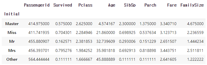
# 위 작업으로 간단하게 그룹화되었는지 확인
- groupby를 통해 Initial Feature에 대한 데이터 현황 출력. 각 Feature에 따른 평균값(mean) 출력
- 타이틀별 평균 나이
→ Master = 5살, Miss = 22살, Mr = 33살, Mrs = 36살, Other = 46살
df_train.groupby('Initial').mean()
>>
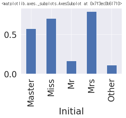
# Initial 에 따른 생존률을 차트로 출력 (통계치 차트)
아래 결과를 보면, 여성(Miss, Mrs)가 남성보다 생존률이 더 높다는 것을 확인할 수 있다.
df_train.groupby('Initial')['Survived'].mean().plot.bar()
>>
반응형
# 위 데이터들을 바탕으로 Age의 Null data 채우기
- Null data를 채울 때는 train dataset 기반으로 산출된 통계치를 train과 test dataset 내 결측값에 채운다.
# Train dataset - Age의 Null data 채우기(그룹별 평균나이로 치환)
df_train.loc[(df_train['Age'].isnull()) & (df_train['Initial'] == 'Mr'), 'Age'] = 33
df_train.loc[(df_train['Age'].isnull()) & (df_train['Initial'] == 'Mrs'), 'Age'] = 36
df_train.loc[(df_train['Age'].isnull()) & (df_train['Initial'] == 'Master'), 'Age'] = 5
df_train.loc[(df_train['Age'].isnull()) & (df_train['Initial'] == 'Miss'), 'Age'] = 22
df_train.loc[(df_train['Age'].isnull()) & (df_train['Initial'] == 'Other'), 'Age'] = 46

# Test dataset에도 동일하게 적용하기
df_test.loc[(df_test['Age'].isnull()) & (df_test['Initial'] == 'Mr'), 'Age'] = 33
df_test.loc[(df_test['Age'].isnull()) & (df_test['Initial'] == 'Mrs'), 'Age'] = 36
df_test.loc[(df_test['Age'].isnull()) & (df_test['Initial'] == 'Master'), 'Age'] = 5
df_test.loc[(df_test['Age'].isnull()) & (df_test['Initial'] == 'Miss'), 'Age'] = 22
df_test.loc[(df_test['Age'].isnull()) & (df_test['Initial'] == 'Other'), 'Age'] = 46
- df_train.loc[(df_train['Age'].isnull()), : ] : "Age = Nan"인 결측값이 있는 경우만 출력
- df_train.loc[(df_train['Age'].isnull()) & (df_train['initial'] == 'Mr'), : ]
: Age에 결측값이 있으면서 Mr 인 데이터만 추출
- df_train.loc[(df_train['Age'].isnull()) & (df_train['initial'] == 'Mr'), 'Age' ]
: 위 조건에서 Age Feature만 추출
- df_train.loc[(df_train['Age'].isnull()) & (df_train['initial'] == 'Mr'), 'Age' ] = 33
: Mr인 Age 결측값은 33살로 입력
+) df_train.loc[(df_train['initial'] == 'Mr'), 'Age' ].isnull().sum()
: Mr인 사람의 Age 값만 추출하고 그 값들 중, Null값이 있는지 확인 ( Null data 여부 확인 )
1.2. Categoized Age 생성
- Continuous한 데이터인 Age를 각 구간별로 카테고리화(Categoized) 시켜서 더욱 학습이 잘 될 수 있도록!
- 하드코딩이 아닌 함수를 사용해서 쉽게 코딩!
# 카레고리화(category_age) 시키는 함수 선언
def category_age(x):
  if x < 10:
    return 0
  elif x < 20:
    return 1
  elif x < 30:
    return 2
  elif x < 40:
    return 3
  elif x < 50:
    return 4
  elif x < 60:
    return 5
  elif x < 70:
    return 6
  else:
    return 7
# 위에 정의한 함수를 'Age'에 적용 - apply()
- apply() 함수를 통해 본인이 정의한 함수를 적용시킬 수 있다.
- Train과 Test dataset에 모두 적용
df_train['Age'].apply(category_age)
df_test['Age'].apply(category_age)
>>
0      2
1      3
2      2
3      3
4      3
      ..
886    2
887    1
888    2
889    2
890    3
Name: Age, Length: 891, dtype: int64
# 적용하기 및 결과 확인
df_train['Age'] = df_train['Age'].apply(category_age)
df_test['Age'] = df_test['Age'].apply(category_age)
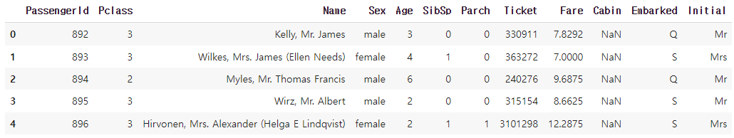
# test dataset에 적용된 결과 확인
df_test.head()
>>
1.3. Embarked
- 'Embarked' 라는 Feature 내 Null data를 확인하고, 가장 많은 데이터로 치환!
# Embarked에 Null data 갯수 확인
- 결측값(Null data)는 총 2개 확인
df_train['Embarked'].isnull().sum()
>>
2
# Null 값은 가장 많은 데이터로 치환
- 총 891개의 row 중, 가장 많은 데이터인 'S'로 결측값 치환
df_train.shape
>>
(891, 14)
# 가장 많은 데이터(S)로 치환
df_train['Embarked'].fillna('S', inplace=True)
# Null data 채워진 것 확인
- '0' 이 출력되는 것으로 보아, Null data가 잘 처리된 것을 확인할 수 있다.
df_train['Embarked'].isnull().sum()
>>
0
// 여기까지 결측값(Null) 처리하는 기본적인 단계를 마치며, 다음 포스팅부터는 또 다른 Feature Engineering을 이어서 수행 예정!
'Data Analyst > Kaggle & DACON' 카테고리의 다른 글
| [Titanic] Model Development(ML) - Randomforest (지도학습) (0) | 2022.12.04 |
|---|---|
| [Titanic] Feature Engineering(2) - One hot encoding, correlation (0) | 2022.11.29 |
| [Titanic] EDA (Exploratory Data Analysis) - 타이타닉 데이터 분석(2) (0) | 2022.10.07 |
| [Titanic] EDA (Exploratory Data Analysis) - 타이타닉 데이터 분석(1) (0) | 2022.10.06 |
| [Titanic] Dataset Check (Train & Test dataset, Null data) - 생존자 예측 (0) | 2022.09.24 |


댓글