(Regression) Ridge Code 실습 및 예제 (Regularized Model)
728x90
반응형
# 학습 목적
1. Linear Regression
- 단순 Linear Regression을 활용하여 변수의 중요도 및 방향성을 알아봄
- 매우 심플한 모델이기 때문에 사이즈가 큰 데이터에 적합하지 않음
→ 하지만, 설명력(해석력)이 큰 장점이 있음
2. Ridge Regression
- Regularized Linear Model을 활용하여 Overfitting을 방지함
→ Ridge Regression은 'L2 norm'을 사용해서 selection은 안되지만, β의 값을 계속 낮출 수 있다.
- Hyperparameter lamba를 튜닝할 때 for loop 뿐만 아니라 GridsearchCV를 통해 돌출
→ CV : Cross Validation의 약자로 'K-fold'를 지정하여 데이터로 나누어서 Overfitting를 최소화하면서 모델의 performance를 측정
3. Regularized Linear Model의 경우, X's Scaling을 필수적으로 진행
# Process
1) Define X's & Y
→ 데이터를 가져와서 X와 Y를 정의
2) Split Train & Valid dataset
→ Train과 Validation set으로 분리. 8:2 혹은 7:3 비중으로 많이 씀
3) Modeling
4) Model 해석
Ridge Regression Code 실습
1. Define X's & Yfd
1) 필요한 패키지 import
# Package 불러오기
import numpy as np
import pandas as pd
from sklearn.model_selection import train_test_split
from sklearn.linear_model import LinearRegression
from sklearn.linear_model import Ridge, RidgeCV
from sklearn.model_selection import GridSearchCV
from sklearn.preprocessing import MinMaxScaler
from sklearn.metrics import mean_squared_error

# Sklearn Toy Data
from sklearn.datasets import load_diabetes
- from sklearn.model_selection import train_test_split
: Data를 split하는 패키지
- from sklearn.preprocessing import MinMaxScaler
: scaling을 하기 위한 패키지
- LinearRegression Ridge, GridSearchCV, MSE 등을 사용하기 위한 패키지 import
# Standard Scaling vs MinMaxScaling
1) Standard Scaling (SS)
: 0을 중심으로 scaling을 하는 방식
2) MinMaxScaling (MS)
: 데이터의 Noise가 없을 때 장점이 크다. Feature의 Min과 Max를 다루는데, 둘 중 한쪽이 지나치게 높지 않아야 원활하게 scaling이 진행될 수 있다.
# Dataset은 sklearn에 있는 샘플데이터를 활용 (당뇨병)
→ from sklearn.datasets import load_diabetes
2) 데이터 살펴보기
# Data Loading (당뇨병 데이터셋 불러오기)
data = load_diabetes()
# 데이터의 shape 확인
print('>>>>X Shape : {}'.format(data['data'].shape))
print('>>>>Y Shape : {}'.format(data['target'].shape))
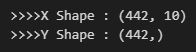
data['data']는 독립변수인 X를 의미하고, data['target']은 종속변수인 Y로 인식한다.
# 데이터 설명 (description)
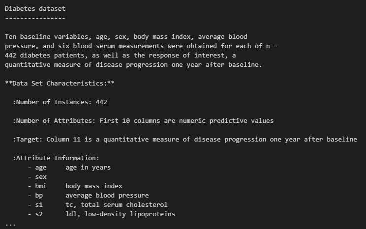
데이터의 Description('DESCR')을 불러오면 Dataset에 대한 설명을 확인할 수 있다.
→ Source URL과 information도 확인 가능
→ target(Y)는 1년 후의 당뇨병 진행상태를 예측한 데이터 (Regression problem)
# 데이터 설명(description)
print(data['DESCR'])
# DataFrame 살펴보기
pd.DataFrame(data['data'], columns=data['feature_names']).describe().applymap(lambda x: f"{x:0.2f}")
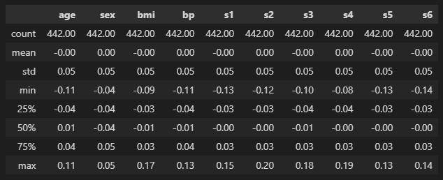
age(첫번째 컬럼)임에도 min값이 -0.11, max값은 0.11이고 성별(sex)도 0 또는 1이 아니고 모두 scaling이 되어있는 상태인 것을 확인할 수 있다.
→ simple linear regression을 할때는 scaling 작업이 해석력을 다소 떨어뜨릴 수 있는데, 위의 데이터들은 이미 scaling이 되어있는 것으로 해석할 수 있다.
→ 따라서 sklearn에서는 column명만 참고하고 데이터는 직접 URL을 통해서 불러와서 실습해보자
# 데이터 불러오기 (URL을 통해서)
pandas에서 read_csv('링크')를 통해서 해당 링크에 있는 데이터를 그대로 불러올 수 있다.
# URL을 통해 데이터 불러오기
data = pd.read_csv('https://www4.stat.ncsu.edu/~boos/var.select/diabetes.tab.txt',sep='\t')

# 데이터 description
data.describe()
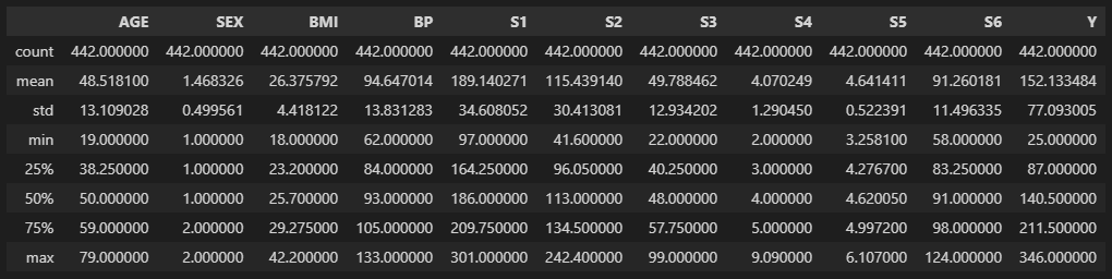
위의 경우에는 나이(AGE)와 성별(SEX) 등의 데이터가 비교적 정상적으로 들어온 것을 확인할 수 있다.
해당 데이터를 활용하여 특정 사람의 1년 후 당뇨병이 어느 정도 진행상태를 보이는지 Y(target)을 예측하는 실습을 진행해보자.
반응형
2. Split Train & Valid dataset
Data Split을 진행할 때 BigData의 경우, 꼭 indexing을 추출하여 모델에 적용시켜야 한다
→ Data Split을 해서 새로운 Data set을 만들 경우, 메모리에 부담을 주기 때문
ex)
X_train = X.iloc[dd]
X_Valid = X.iloc[dd]
→ 이 경우, X를 2번이나 선언한 것이기에 데이터가 많은 경우 메모리에 무리가 갈수도 있다
1) X's & Y Split
# Data Split
# X's & Y Split
Y = data['Y']
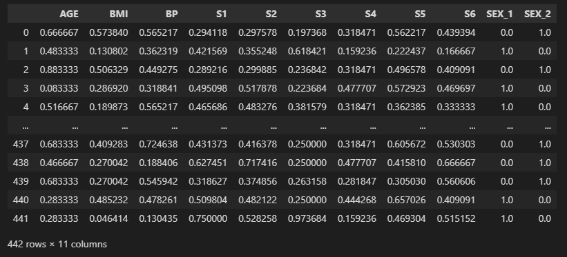
X = data.drop(columns=['Y'])
X = pd.get_dummies(X, columns=['SEX'])위와 같이 X와 Y를 분리시키고, 성별(SEX)에 대해서 1과 2로 정보가 구분되어있는데 이는 categorical 변수이므로 dummy variable로 바꿔서 저장하는 것이 좋다.
→ 만약, 성별(SEX)를 1과 2로만 구분한다면, 데이터는 2가 1보다 크다고만 인식을 하게 된다.

SEX (categorical 변수) 데이터를 dummy variable로 저장하면, 위의 결과와 같이 SEX_1과 SEX_2로 dummy로 쉽게 구분할 수 있게 된다.
2) Training / Validation set split
# Training set과 Validation set 분리
idx = list(range(X.shape[0]))
train_idx, valid_idx = train_test_split(idx, test_size=0.3, random_state=2024)
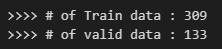
print(">>>> # of Train data : {}".format(len(train_idx)))
print(">>>> # of valid data : {}".format(len(valid_idx)))
- idx = list(range(X.shape[0])
: X.shape[0] : (442, 11) 이므로 이를 활용하여, 442개의 list를 생성해서 index 추출하고 split
- train_idx, valid_idx = train_test_split(idx, test_size=0.3, random_state=2024)
: 그리고 그 index를 train과 valid에 맞게 split을 해준다.
→ 여기서의 test size는 0.3이므로, 7:3의 비율로 분리
→ 학습할 때마다 index가 변경되는 것을 방지하기 위해
3. Modeling (Linear Regression)
그럼 이제부터 Linear Regression을 진행해보자
→ Model fitting할 때는 X값이 아닌 index값을 넣어주자
1) Model fitting
# Linear Regression
results = LinearRegression().fit(X.iloc[train_idx], Y.iloc[train_idx])
Model fitting할 때는 X값을 넣어주는 것이 아닌 데이터의 index를 넣어주자
→ 따로 데이터를 만들지 않아도 모델 학습이 가능하다
→ 데이터가 많을수록 이 방식이 유리하다
2) 해석을 위한 함수 선언
LinearRegression은 내장함수가 데이터를 해석하는데 많은 도움이 되지는 않는다.
→ summary 해주는 함수가 따로 없기 때문에 별도로 추출해서 해석을 해야하는 번거로움이 있다.
→ 그래서 깔끔하게 해석을 위한 함수를 생성하면 더 좋다.
import scipy
from sklearn import metrics

def sse(clf, X, y):
    """Calculate the standard squared error of the model.
    Parameters
    ----------
    clf : sklearn.linear_model
        A scikit-learn linear model classifier with a `predict()` method.
    X : numpy.ndarray
        Training data used to fit the classifier.
    y : numpy.ndarray
        Target training values, of shape = [n_samples].
    Returns
    -------
    float
        The standard squared error of the model.
    """
    y_hat = clf.predict(X)
    sse = np.sum((y_hat - y) ** 2)
    return sse / X.shape[0]


def adj_r2_score(clf, X, y):
    """Calculate the adjusted :math:`R^2` of the model.
    Parameters
    ----------
    clf : sklearn.linear_model
        A scikit-learn linear model classifier with a `predict()` method.
    X : numpy.ndarray
        Training data used to fit the classifier.
    y : numpy.ndarray
        Target training values, of shape = [n_samples].
    Returns
    -------
    float
        The adjusted :math:`R^2` of the model.
    """
    n = X.shape[0]  # Number of observations
    p = X.shape[1]  # Number of features
    r_squared = metrics.r2_score(y, clf.predict(X))
    return 1 - (1 - r_squared) * ((n - 1) / (n - p - 1))


def coef_se(clf, X, y):
    """Calculate standard error for beta coefficients.
    Parameters
    ----------
    clf : sklearn.linear_model
        A scikit-learn linear model classifier with a `predict()` method.
    X : numpy.ndarray
        Training data used to fit the classifier.
    y : numpy.ndarray
        Target training values, of shape = [n_samples].
    Returns
    -------
    numpy.ndarray
        An array of standard errors for the beta coefficients.
    """
    n = X.shape[0]
    X1 = np.hstack((np.ones((n, 1)), np.matrix(X)))
    se_matrix = scipy.linalg.sqrtm(
        metrics.mean_squared_error(y, clf.predict(X)) *
        np.linalg.inv(X1.T * X1)
    )
    return np.diagonal(se_matrix)


def coef_tval(clf, X, y):
    """Calculate t-statistic for beta coefficients.
    Parameters
    ----------
    clf : sklearn.linear_model
        A scikit-learn linear model classifier with a `predict()` method.
    X : numpy.ndarray
        Training data used to fit the classifier.
    y : numpy.ndarray
        Target training values, of shape = [n_samples].
    Returns
    -------
    numpy.ndarray
        An array of t-statistic values.
    """
    a = np.array(clf.intercept_ / coef_se(clf, X, y)[0])
    b = np.array(clf.coef_ / coef_se(clf, X, y)[1:])
    return np.append(a, b)


def coef_pval(clf, X, y):
    """Calculate p-values for beta coefficients.
    Parameters
    ----------
    clf : sklearn.linear_model
        A scikit-learn linear model classifier with a `predict()` method.
    X : numpy.ndarray
        Training data used to fit the classifier.
    y : numpy.ndarray
        Target training values, of shape = [n_samples].
    Returns
    -------
    numpy.ndarray
        An array of p-values.
    """
    n = X.shape[0]
    t = coef_tval(clf, X, y)
    p = 2 * (1 - scipy.stats.t.cdf(abs(t), n - 1))
    return p

def summary(clf, X, y, xlabels=None):
    """
    Output summary statistics for a fitted regression model.
    Parameters
    ----------
    clf : sklearn.linear_model
        A scikit-learn linear model classifier with a `predict()` method.
    X : numpy.ndarray
        Training data used to fit the classifier.
    y : numpy.ndarray
        Target training values, of shape = [n_samples].
    xlabels : list, tuple
        The labels for the predictors.
    """
    # Check and/or make xlabels
    ncols = X.shape[1]
    if xlabels is None:
        xlabels = np.array(
            ['x{0}'.format(i) for i in range(1, ncols + 1)], dtype='str')
    elif isinstance(xlabels, (tuple, list)):
        xlabels = np.array(xlabels, dtype='str')
    # Make sure dims of xlabels matches dims of X
    if xlabels.shape[0] != ncols:
        raise AssertionError(
            "Dimension of xlabels {0} does not match "
            "X {1}.".format(xlabels.shape, X.shape))
    # Create data frame of coefficient estimates and associated stats
    coef_df = pd.DataFrame(
        index=['_intercept'] + list(xlabels),
        columns=['Estimate', 'Std. Error', 't value', 'p value']
    )
    try:
        coef_df['Estimate'] = np.concatenate(
            (np.round(np.array([clf.intercept_]), 6), np.round((clf.coef_), 6)))
    except Exception as e:
        coef_df['Estimate'] = np.concatenate(
            (
                np.round(np.array([clf.intercept_]), 6),
                np.round((clf.coef_), 6)
            ), axis = 1
    )[0,:]
    coef_df['Std. Error'] = np.round(coef_se(clf, X, y), 6)
    coef_df['t value'] = np.round(coef_tval(clf, X, y), 4)
    coef_df['p value'] = np.round(coef_pval(clf, X, y), 6)
    # Output results
    print('Coefficients:')
    print(coef_df.to_string(index=True))
    print('---')
    print('R-squared:  {0:.6f},    Adjusted R-squared:  {1:.6f},    MSE: {2:.1f}'.format(
        metrics.r2_score(y, clf.predict(X)), adj_r2_score(clf, X, y), sse(clf, X, y)))
ex)
- sse(clf, X, y)
: MSE를 함수로 표현한 것. clf에 모델을 넣고, X와 y값을 넣어주게 되면 모델이 prediction한 결과값인 y_hat을 추출할 수 있다. 그리고 그 'y_hat'값과 실제 True값(y)와의 차이로 MSE로 구할 수 있다.
→ X.shape[0] : 데이터의 갯수
→ X.shape : [Row 갯수, Column 갯수]
3) Summary
위에서 선언한 함수들을 통해 summary 함수를 돌려보면
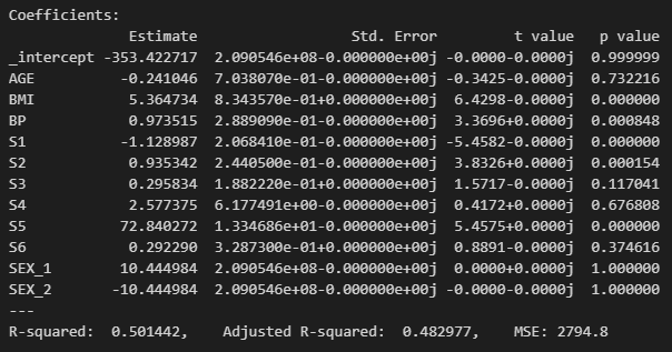
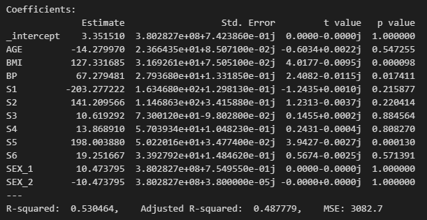
summary(results, X.iloc[valid_idx], Y.iloc[valid_idx], xlabels=X.columns)

X에 대한 valid data를 가지고 결과를 보면, 위의 결과처럼 R-squared값이 '0.53'으로 꽤 높은 수치이다.
→ 보통 R-square값이 0.25 정도면 사용이 가능하다. 0.53이면? 굉장히 유의미한 결과라고 볼 수 있다.
# 해석 순서
1) R-square값 보기
: 0.25 이상이어야 사용할만한 데이터라고 판단!
2) p-value
: 기울기가 0이 아닐 확률! '0.05' 보다 작으면 통상적으로 유의미하다고 볼 수 있다.
→ 위에서는 S2가 꽤 유의미하다고 해석할 수 있다.
여러 Feature들 중에서 어떤 변수들이 유의미한지를 파악했다면, 이제 y값에 얼마만큼의 영향을 미치는지를
확인해야 한다.
→ BMI의 경우 1단위 증가했을 때, 당노병 progress에 '5.36'만큼의 영향을 준다고 해석할 수 있다.
→ 마찬가지로 S5는 1단위 증가분에 따라 '72'만큼의 영향을 준다고 볼 수 있다.
하지만, 위와 같은 해석만을 두고 어떤 변수가 더 중요한지는 판단할 수 없다.
→ 그래서 특정 결과에 도출하는 데에 여러 변수들 중에서 어떤 변수가 중요한지 판가름하는 법을 숙지할 필요가 있다.
왜? 각 변수의 증가분에 따라 결과값에 미치는 가중치가 다르기 때문이다.
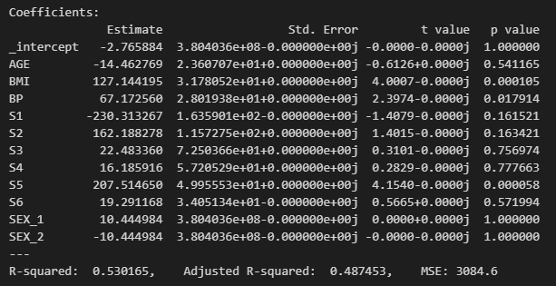
summary(results, X.iloc[train_idx], Y.iloc[train_idx], xlabels=X.columns)
위의 결과는 validation이 아닌 training set에서 구한 결과이다.
→ training set보다 validation set의 R-squared값이 높다는 것은 overfitting이 안되었다는 의미!
4) Scaling
# Scaling
scaler = MinMaxScaler().fit(X.iloc[train_idx])
X_scal = scaler.transform(X)
X_scal = pd.DataFrame(X_scal, columns=X.columns)
X를 가지고 Scaling을 진행 (MinMaxScaler)
→ fit()을 할 때, training index로만 수행. 모든 X의 70% 정도만 Scaler
→ transform은 모든 X에 대해서 수행. 변환시킬 때는 모든 X에 적용되어야 한다.
X_scal
위와 같이 X training index에 Scaling이 잘 된 것을 확인할 수 있다.
→ 모든 값이 0과 1 사이의 값으로 정렬됨
4. Model 해석
# Linear Regression
results = LinearRegression().fit(X_scal.iloc[train_idx], Y.iloc[train_idx])
summary(results, X_scal.iloc[valid_idx], Y.iloc[valid_idx], xlabels=X_scal.columns)
Scaling까지 한 후의 summary를 보면, p-value는 거의 동일하고 BMI, BP, S1, S2, S5가 유의미하다고 볼 수 있다.
→ Scaling까지 한 후의 해석을 해보면, 이제 어느 변수가 중요한지 판단할 수 있다. S5.
'S5 → BMI → S1' 순으로 중요하다고 볼 수 있다.
왜냐하면? Scaling으로 모두 변수의 1단위 증가에 따른 가중치를 동일하게 두었기 때문에,
Scaling 이후의 결과를 통해 어느 변수가 결과에 제일 많은 영향을 끼치기 때문에 가장 중요한지를 판단할 수 있다.
5. Ridge Regression
'for loop'와 'GridSearchCV'를 통해 파라미터 tuning하고, ridge regression하는 법에 대해 알아보자.
1) for loop을 통한 Ridge
[Ridge Regression Parameters]
- Package : https://scikit-learn.org/stable/modules/generated/sklearn.linear_model.Ridge.html
- alpha : L2-norm Penalty Term
→ alpha : 0 일 때, Just Linear Regression
- fit_intercept : Centering to zero
→ 베타0를 0로 보내는 것 (베타0는 상수이기 때문에)
→ 베타0은 딱히 의미가 없기 때문에
- max_iter : Maximum number of interation
→ Loss Function의 Ridge Penalty Term은 Closed Form 값이기는 하지만 값을 찾아 나감
→ Penalty Term : (1 / (2 * n_samples)) * ||y - Xw||^2_2 + alpha * ||w||_2
penelty = [0.00001, 0.00005, 0.0001, 0.001, 0.01, 0.1, 0.3, 0.5, 0.6, 0.7, 0.9, 1, 10]

# Using For Loop !!
# Ridge Regression
# select alpha by checking R2, MSE, RMSE
for a in penelty:
    model = Ridge(alpha=a).fit(X_scal.iloc[train_idx], Y.iloc[train_idx])
    score = model.score(X_scal.iloc[valid_idx], Y.iloc[valid_idx])
    pred_y = model.predict(X_scal.iloc[valid_idx])
    mse = mean_squared_error(Y.iloc[valid_idx], pred_y)
    print("Alpha:{0:.5f}, R2:{1:.7f}, MSE:{2:.7f}, RMSE:{3:.7f}".format(a, score, mse, np.sqrt(mse)))
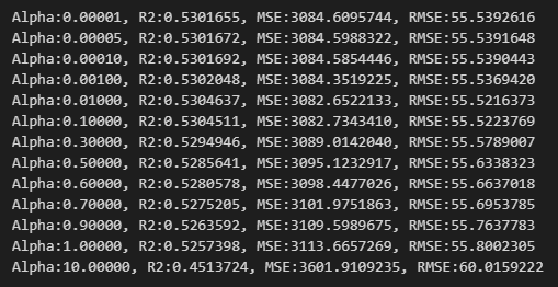
먼저 penalty에 대한 리스트를 생성하고, Model을 Ridge에 알파를 계속 넣어줌(for loop)으로써 fitting을 시켜준다.
→ 이때 Scaling한 training data 넣어주고
→ 여기서의 'model.score'는 R-squared값.
→ 예상한 y값(pred_y)를 산출 후, MSE도 계산. 그리고 여기에 루트를 씌우면 RMSE가 된다.
이 과정을 통해, Alpha, R2, MSE, RMSE를 통해 해석을 해보면
Alpha가 '0.01'일 때, R2(=R-squared값)이 제일 높고(0.5304637), RMSE가 55.52값으로 제일 낮기 때문에 Alpha를 0.01로 선택하면 된다.
model_best = Ridge(alpha=0.01).fit(X_scal.iloc[train_idx], Y.iloc[train_idx])
summary(model_best, X_scal.iloc[valid_idx], Y.iloc[valid_idx], xlabels = X_scal.columns)
위에서 선택한 Alpha '0.01' 값을 넣어주고, Ridge regression을 돌려보면 기본 Linear regression을 돌린 결과와 큰 차이는 없다. 다소 높은 성능을 보이는 정도?
→ Linear : 0.5301 (=53.01%)
→ Ridge : 0.5304 (=53.04%)
2) GridSearchCV
위에서 선언한 penalty를 가지고 이번엔 GridSearchCV 방법으로 Ridge를 돌려보자
→ penelty = [0.00001, 0.00005, 0.0001, 0.001, 0.01, 0.1, 0.3, 0.5, 0.6, 0.7, 0.9, 1, 10]
# Using GridSearchCV
ridge_cv=RidgeCV(alphas=penelty, cv=5)
model = ridge_cv.fit(X_scal.iloc[train_idx], Y.iloc[train_idx])
print("Best Alpha:{0:.5f}, R2:{1:.4f}".format(model.alpha_, model.best_score_))
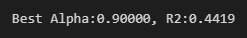
CV를 돌렸을 때는 결과값이 Alpha가 0.9일때, R2값이 0.4419라고 나와서 'for loop'를 돌렸을 때의 값들과 상이한 점에서 조금 이상할 수 있다. 그래서 이번엔 GridSearchCV를 통해 돌릴 수 있는 것만 확인하는 정도로 학습하자.
# GridSearchCV Result
model_best = Ridge(alpha=model.alpha_).fit(X_scal.iloc[train_idx], Y.iloc[train_idx])
score = model_best.score(X_scal.iloc[valid_idx], Y.iloc[valid_idx])
pred_y = model_best.predict(X_scal.iloc[valid_idx])
mse = np.sqrt(mean_squared_error(Y.iloc[valid_idx], pred_y))
print("Alpha:{0:.5f}, R2:{1:.7f}, MSE:{2:.7f}, RMSE:{3:.7f}".format(0.01, score, mse, np.sqrt(mse)))
summary(model_best, X_scal.iloc[valid_idx], Y.iloc[valid_idx], xlabels=X_scal.columns)
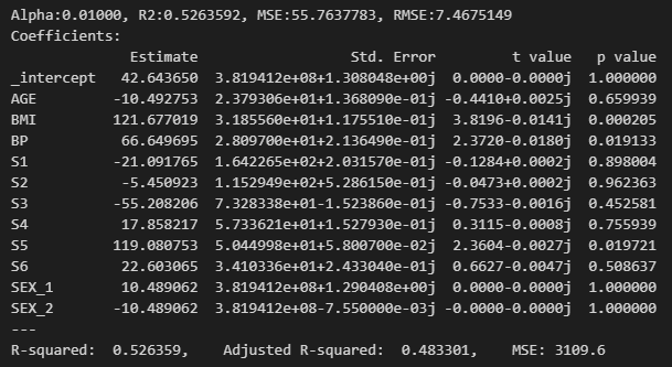
위와 같이 결과를 확인할 수 있다.
'for loop'와 'GridSearchCV'는 사용자의 기호에 맞게 사용하면 된다.
주로 원하는 결과값을 선택해서 사용하는 것을 더 선호한다면 'for loop'가 더 알맞은 방법일 수 있다.
'Machine Learning > Regression Problem' 카테고리의 다른 글
| (Regression) LASSO 기초 정리 (Ridge와 차이점은?) (0) | 2024.07.04 |
|---|---|
| (Regression) Ridge regression 쉬운 풀이! (Regularized Model) (0) | 2024.07.02 |
| (Regression) Feature selection을 보완한 기법, 'Penalty Term'이란? (0) | 2024.04.10 |
| (Regression) Overfitting 방지하는 Feature Selection 기법의 종류 정리 (0) | 2024.04.07 |
| (Regression) Model 평가 및 지표 해석하는 방법! - 성능지표 총 정리 (0) | 2024.04.05 |


댓글